Q-Day
"Mathematicians that lack imagination become poets..." - Bronislovas Burgis
Tuesday, 27 January 2015
RWE npower Forecasting Challenge (mind the amended e-mail)
Recently, I asked a few people from quant and forecasting teams to try the task out in order to validate the data and get some opinions about the difficulty of it. What happened is that after few attempts it was clear that half-hourly data might be a bit too detailed for 2nd or 3rd year student. I don't think I have seen a dataset with more than 500 observations during my undergrad while data had 70000.
Finally it was agreed to aggregate the data to daily granularity and we tested it again. This time I got forecasts promptly and noticed that some competition is arising internally. This has led to allowing internal applicants to attempt the task. It was agreed that main competition rating ta able will be kept separate, but all applicants including internal will have a separate one - I bet graduates will also be interested how well they did against someone who is actually working in forecasting.
Finally, I thought that it doesn't make much effort to also allow external non-student participants. Thus we agreed that anyone can apply.
The task is quite simple:
Train on 2 years, provide forecasts for next 6 months.
Then get actuals for those 6 months, train again, forecast for next 6 months.
And do the same again.
Total 3 rounds, measure is MAPE - mean(abs(percentage error)).
I quite enjoyed attempting the task myself and having unfair advantage of being able to test on actuals outperformed everybody. However, the same model has performed even better in rounds 2 and 3 without any further adjustments.
I don't think it would take more than an hour for somebody who knows his/her R and might be a good fun seeing yourself against results of internal RWE npower forecasting team, internal quants and most importantly graduate students! :)
"Please note this competition is for University students only (see terms & conditions). However if you would still be interested
in attempting the challenge please email graduates@RWEnpower.com. You will not be eligible for the prize but your forecast will be scored and appear in our rankings."
Note amended e-mail!
For more information visit: http://www.npowerjobs.com/graduates/forecasting-challenge-2015
Good luck in forecasting and hope to see you in high scores!
By the way this is how my first train model looked like. (Different dataset though)
Sunday, 7 July 2013
Variance Swap Replication in R.
As I was studying volatility derivatives I made some charts that represent some key features of replication. Say variance swap has a payoff function \(f=(\sigma - K_{VOL}) \), which means that \(K_{VOL}\) will most likely be the forward volatility close to implied. To replicate this theory goes deep into maths and log-contracts that are not even traded on the market, however the idea is simple, buy a portfolio of options with equally distributed strike prices and weight them by reciprocal of squared strikes, i.e.\( 1 \big/ K^2 \). Go for liquid ones, i.e. out of the money puts and out of the money calls. Then volatility or in this case variance is dependent on VEGA sensitivity of portfolio. The following graph gives an idea of how it is done. The code is included below:
X-Y - spot/time to maturity, Z - Vega \( \left(\frac{\partial C}{\partial \sigma}\right) \).
vega <- function(S0=100, K=100, r=0.05, d=0.05, tau=1, vol=0.1){ d_1 <- (log(S0/K)+((r-d)+vol^2/2)*tau)/(vol*sqrt(tau)); S0*sqrt(tau)*(1/sqrt(2*pi)*exp(-d_1^2/2))*exp(-d*tau)} vegaK <- function(K, t){ sapply(t, function(x){vega(S0=50:200, K=K, tau=x)/K^2}) } my3d_plot <- function(mat, x, y, col, bgcol="slatergray", material="lines", add=FALSE, ...){ require(rgl); if( missing(x) ){ x <- 1:nrow(mat) }; if( missing(y) ){ y <- 1:ncol(mat) } if( missing(col) ){ col <- rev(rep(heat.colors(ncol(mat),alpha=0),each=nrow(mat))) } if( !add ){ open3d(); material3d(color=bgcol) } persp3d(x, y, mat, col = col, alpha=1, front=material, back=material, add=add, ...)} mat <- lapply(seq(60,180,15), vegaK, t=seq(1,0,length=20)) mat$sum <- Reduce("+", mat) my3d_plot(mat$sum, bgcol="white", col="grey", aspect=c(4, 3, 2)) sapply(mat[1:9], my3d_plot, col="green", add=TRUE)
Wednesday, 26 June 2013
Technical(and not technical) strategy testing
Now to begin I would like to reason why I have done this while there exist a nice "blotter" and "quantstrat" packages.
First of all "quantstrat" is faster than blotter, which is good. However it was not good enough for me. Once you have 1 minute data and you want to optimise a strategy on 1 year data you can leave your code running for a few days, what is not very convenient as your strategy could be worth absolutely nothing while spending so much time on it. I would also like to note, that the bigger the matrix, the slower the script runs, speaking in relative terms of course. And this is general tendency for R. So I found that 1 minute data is best to test on 1 month minute data without causing too much inconvenience. Of course you will not get away with it once you found a good strategy... and really hurts to see how your code slows down by a significant multiplier once you double the size of your observations. Solution might be to split your data into parts(which just came to my mind while writing this), but then you loose few trades and have to work out your reconstruction, which might be messy with a slight loss in testing "robustness".
Secondly, I want to tell what I think the advantages against Meta stock or other backtesting software are. Answer is simple: machine learning, garch, nlm, no limits. Disadvantages: loss of speed. Another idea which just came to my mind is to write the main loop in Cpp! And given my approach it is feasible!
And my approach is simple and similar to "quantstrat". Also I got few ideas from my friend who is using Meta Stock(in terms of structuring my code). The speed benefit comes from the fact that it is maintained as simple as possible to get the required result.
GIT REPOSITORY:
https://github.com/afraid2trade/fast_strat.git
So lets see an example. Gist is embedded above, however I will explain it in some detail:
1. load your data with OHLC(column names will be converted to "open", "high", "open", "close" for simplicity.
data = dbase(0, 1)
X = to.minutes(data)["201201"]
> dim(X)
[1] 31680 4
2. initialise your reference main class:
stra = Strat(data=X)
args(Strat)
function (data, init = 10000, qty = 5 * init, spread = 2)
data - OHLC (xts class)
qty - trading position
spread - FX spread
> class(stra)
[1] "tstrat"
23 methods, of which 11 are possibly relevant:
ind, l.entry, l.exit, names, plot, run, s.entry, s.exit, signal, time
ind - add your indicator
signal - define your signal
time - on which weekdays and at what time you want to trade
> args(stra$time)
function (from = 0, to = 23, days = 2:6)
l.entry, l.exit, s.entry, s.exit - all have same arguments
> args(stra$l.entry)
function (columns, true)
columns - names of columns of signals
true - vector of TRUE FALSE indicating which signals you prefer true, which false
3. Add your indicators:
stra$ind(fun=SMA, name="smaf", n=20, prefun=Cl)
stra$ind(fun=SMA, name="smas", n=50, prefun=Cl)
4. Add your signals:
stra$signal(name="crossup", type="cross", col1="smaf", col2="smas")
stra$signal(name="crossdown", type="cross", col1="smas", col2="smaf")
5. Add your entry exit conditions based on signals:
stra$l.entry("crossup",1)
stra$l.exit("crossdown",1)
stra$s.entry("crossdown",1)
stra$s.exit("crossup",1)
6. Run the code! Note the dimensions of given "X" matrix.
stra$run()
On my 3 year old macbook pro it took no more than 3 minutes(given that matlab inbuilt test rated my laptop performance to be lowest among all benchmarks it looks good. doesnt it?)
This is a result of the fact that in the loop I used as little objects as possible and have split them to multiple matrices to reduce their size what makes R deal with them faster.
7. Plot results!
stra$plot()
addSMA(20)
addSMA(50)
It contains:
a) charted series with red dots where trades has occurred
b) wealth index
c) position at the time
8. Your data with all indicators, returns, etc can be accessed:
stra$data
str(stra$data)
ret = stra$data$ret
Good things(as Q&A):
1. How many lines I need to do all of this? 16(including 1 line to initialise and 2 lines to load the data).
2. Do I have numerous arguments for each function? No.
3. Does the framework work? Try yourself.
Bad things:
I lost 80% of my initial capital with this strategy.
That is about it. Looks simple, but you can do anything you want without complicated structures. What I mean is I liked "quantstrat", however it took me few days to grasp what is going. Also, it has a lot of functionality that I have not used and finally functionality that I wanted to use was not there, while now I have my simple code that I can manipulate.
source("/Users/Edu/core/Projects/fast_strat/0_fstrat_init.R") # load all data <- dbase(0, 1) # my own written function for database X <- to.minutes(data)["201201"] #### TEST ######################## stra <- Strat(data=X) # initialise stra$ind(fun=SMA, name="smaf", n=20, prefun=Cl) stra$ind(fun=SMA, name="smas", n=50, prefun=Cl) stra$signal(name="crossup", type="cross", col1="smaf", col2="smas") stra$signal(name="crossdown", type="cross", col1="smas", col2="smaf") stra$l.entry("crossup",1) stra$l.exit("crossdown",1) stra$s.entry("crossdown",1) stra$s.exit("crossup",1) stra$run() stra$plot() addSMA(20) addSMA(50)
My plans for future regarding this little project:
1. Add simple stop loss methods.
2. Make it more general in terms of defining tax and spread functions.
3. Include better position management
4. Edit the aggregation of terminal results: i.e. dealing with trading prices(close or next period open, which day P&L will it represent etc)
5. Refine the code to give the right errors in right places
6. Rewrite the terminal loop in Cpp. Loop currently contains 42 lines and might expand to, i think, 60 after stop loss inclusion. Cpp should not take more than 150 lines
Once again, feedback and comments are welcome.
Sunday, 16 June 2013
Scenario analysis and trading options using R
Lets say you are constructing a portfolio. You want to start with risk-reversal strategy(buy call high, sell put low). You are interested in payoff chart:
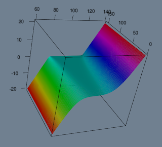
For some reason you decide to short a stock and add it to your portfolio:
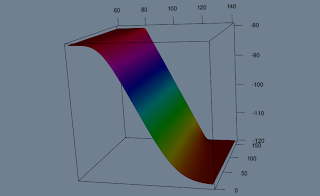
You now realise that you must really have negative view on the market to trade this. You decide that this will be your view, but your neighbour tells you that a sharp price increase is possible. Decide to buy some digitals:
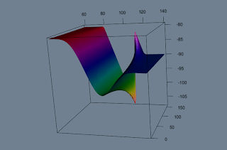
You are satisfied with your decisions and would like to check you profit and loss as up to now numbers on z axis just showed payoff. Remember as you shorted the stock, you've got some cash. In particular 100. But your digitals cost and sum of option prices should be slightly positive as both symmetrically out of the money:
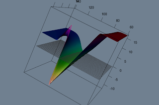
While you are very happy with your decisions you also want to investigate some sensitivities. Say vega:
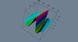
Now you're like:"Not trading this weird thing".
If you liked what you saw and you want to try it yourself or even contribute, continue reading.
"sa_work.R" is the file where you would normally work. It has only 1 line to call all you need:
source("~/core/Projects/scenario_analysis/0_sa_init.R")
This is the only line you need to change once you have repository downloaded. Just locate "0_sa_init.R" and it will do all. And by all I mean 2 things: load packages, load other scripts and couple of basic parameters.
Dependencies:
"quantmod" might be needed if you want to download some option or stock data from yahoo. "RQuantLib" is not currently used, but pricing functions might be taken from it later to price americans. "fields" was used in earlier version for interpolation over scatter and might be needed in later development. "rgl" - 3d graphics. "lubridate" is not essential, but it makes life easier when working with dates at user level. However all date objects are automatically converted to "timeDate" class.
File structure is simple:
"0_funs" folder with 2 scripts loaded from it "0_basic.R" that contains some basic functions - only 2 out of 5 are really needed. And "0_inst.R" - abbreviation for instruments, but now contains all the project within. Surprisingly only 500 lines of code. Went down twice after I drifted to OOP approach.
"2_structure_int.R", "2_structure_vol.R" will be used for interest rate structure and implied volatility surface implementation in the future and are currently not used.
Classes:
Classes used are S4 for outputs, some simple variables that needed formalisation and parameter objects. Reference classes are used for instruments.
S4:
"currency" inherits from "character" and Currency() function makes sure its of length 3 and creates new.
"gen.par" contains number of preferred working days in a year and list of interest rates.(later could be extended to interest rate structure).
"stock.par" contains all parameters that are stock specific and varies over time.
"scatter" inherits from "matrix". Contains output from reference classes: data, row and column variables.
Reference:
"security" superclass of all securities.
"spot", "forward" and "option" inherits from "security".
All of them have same methods: price, delta, gamma, theta, rho, rhoQ, vega. All of them have arguments: st(stock price), tVec(time), vol(volatility). "option" class has additional method: getiv.
Here is the list of functions you need:
time_seq(from, to, by = "hour", rng = c(9, 16), holiday = holidayNYSE(2013:2020), trading = TRUE)
- creates time sequence. All methods round the time to hourly so don't use higher frequency! Also, avoid using daily, just stick to default until you know what you are doing.
GenPar() - creates "gen.par" object named "gen.par" and assigns it to "gen.par" environment.
lsg() gets you gen.par object
StockPar() - analogous to GenPar, just names it paste0(ticker,".par")
lss() - lists objects in "stock.par" environment
rms() - clears "stock.par" environment
Spot(id, num=1, class="equity", cur="usd"),
Forward(id, underlying, maturity, K, num=1, class="equity", cur="usd"),
Option(id, underlying, maturity, K, put, ame=0, type="vanilla", num=1, extra=list(0), class="equity", cur="usd")
- creates security objects and assigns it to "securities" environment.
lsi() - lists objects in "securities" environment
rmi() - clears "securities" environment
vaSecurities() - collects all objects in "securities" environment in a list.
Good news. this is all you need. Few things to note. All strings are converted to CAPS including object names for instruments. Only security class is equity. Only 2 option types are available: "vanilla" and "binary"(cash-or-nothing). All options are european.
source("~/core/Projects/scenario_analysis/0_sa_init.R") ######################################################################## GenPar( rates = list("USD"=0.05), nyear = 252 ) StockPar( ticker = "aapl", # ticker of the stock s0 = 100, # current price of the stock given time(date below) vol = 0.3, # yearly vol(numeric) d = 0, # date = Sys.Date() # converted "timeDate": you can enter this in many formats, say: 20120714 ) ######################################################################## # Spot("AAPL") # Forward("AAPLF", "AAPL", Sys.Date()+days(30), 110) # Option("AAPLC", "AAPL", Sys.Date()+days(30), 100, 0, 0, type="binary", num=1) Spot("AAPL", num= -1) Option("AAPLC", "aapl", Sys.Date()+days(30), 120, 0, 0, type="vanilla", num= 1) Option("AAPLP", "aapl", Sys.Date()+days(30), 80 , 1, 0, type="vanilla", num=-1) Option("AAPLB", "aapl", Sys.Date()+days(30), 110 , 0, 0, type="binary", num=30) t <- time_seq(Sys.Date(),Sys.Date()+2) s <- seq(80,120,10) v <- seq(0.1,0.5,0.1) AAPLC$price() # current price [1,] 0.05804536 AAPLC$delta() # current delta AAPLC$getiv(AAPLC$price()) # [1] 0.3000074 # say you observe the price higher in the market: 0.1! AAPLC$getiv(0.1) # [1] 0.3263369 # assign it to stock parameter! AAPL.par@vol <- AAPLC$getiv(0.1) # you have correct volatility now p1 = AAPLC$price(st=s, tVec=t) # use st with tVec p2 = AAPLC$price(vol=v, tVec=t) # or vol with tVec p3 = AAPLC$price(vol=v, st=s) # DON'T use st with vol str(p1) # Formal class 'scatter' [package ".GlobalEnv"] with 4 slots # ..@ .Data: num [1:5, 1:8] 1.63e-06 8.97e-04 5.80e-02 8.34e-01 4.28 ... # ..@ rows : num [1:5] 80 90 100 110 120 # ..@ rows2: num 0.3 # ..@ cols : num [1:8] 0.0794 0.0789 0.0784 0.0779 0.0774 ... # the output is the same("scatter") from all methods except "getiv" class(p1) # scatter plot(p1) class(p1+20) # scatter b1 = AAPLP$price(st=s, tVec=t) # sum the payoffs class(p1+b1) # matrix - not good plot(p1+b1) # not a good idea class(sum(p1, b1)) # scatter - stick to this plot(sum(p1, b1)) # sum creates new "scatter" object # and all attributes are taken from 1st object! # MEANS: never put a "spot" object first as due to the fact, # that it does not have maturity, time axis will be incorrect! cost <- as.numeric(sum(AAPLC$price(), AAPLP$price(), AAPL$price(), AAPLB$price())) cost # [1] -96.04445 means you have cash! port <- sum(AAPLC$price(s,t), AAPLP$price(s,t), AAPL$price(s,t), AAPLB$price(s,t)) plot(port-cost) # here is your proffit and loss! vega <- sum(AAPLC$vega(s,t), AAPLP$vega(s,t), AAPL$vega(s,t), AAPLB$vega(s,t)) plot(port-cost) # and here is your vega # make parameters longer and finer to generate nice graphs: t <- time_seq(Sys.Date(),Sys.Date()+30) s <- seq(80,120,1) # and repeat
Try it out. Your opinions on flaws, mistakes or improvements are more than welcome.
https://github.com/afraid2trade/SCENARIO_ANALYSIS.git
Thursday, 30 May 2013
Scenario analysis for option strategies.
The idea is to develop accurate scenario analysis on portfolio, which is based on a single underlying. In the past I have written some code on simply plotting the payoffs at maturity, then followed a small piece of code, which was improved in a way that specific date could have been chosen for which the payoff is plotted.
For my current project I think the output will be self explanatory. The code is just the running bit to give a feeling of what it does and how it does what it does:
######################## GEN PARAMETERS ############################### gen.par <- vaGenPar(date.start=Sys.Date(), date.end=Sys.Date()+days(359),r=0.05, cal="UnitedStates") ######################## STOCK PARAMETERS ############################# AAPL <- vaSPar("AAPL", s0=100, date=Sys.Date(), vol=0.3720573) # AMZN <- vaSPar("AMZN", s0=100, date=Sys.Date(), vol=0.4548506) stock.par <- vaStockPar(AAPL) ######################## INSTRUMENTS ################################## rmi() # equity_s("AAPL","USD", num=1) # equity_f("AAPL_fut", "AAPL", "USD", Sys.Date()+days(180), num=1) equity_o("AAPL1", "AAPL", "USD", Sys.Date()+days(360), 80, 0, 0, "vanilla", num=1) equity_o("AAPL2", "AAPL", "USD", Sys.Date()+days(360), 100, 0, 0, "vanilla", num=-2) equity_o("AAPL3", "AAPL", "USD", Sys.Date()+days(360), 120, 0, 0, "vanilla", num=1) instruments <- vaInstruments() ######################## RUN ########################################### output <- main.aggregate(gen.par, stock.par, instruments, nsd=2, step=0.005, nstd=1.5) play3d(spin3d(axis=c(0,0,1), rpm=5), duration=12)
The range of the stock values are 2 standard deviations that were plugged into GBM, which was obviously adjusted for risk neutrality as we are in pricing framework. The red line indicates 1.5 standard deviation line. "step" is increment of possible stock prices via volatility.
Furthermore, it returns a function which does an interpolation over the surface, so analysis at each time point can simply be done.
x=50:300
y=outfun(Sys.Date()+days(185), x)
plot(x,y,"l")
For now, the interest rates used are flat as well as implied volatility surface. However, the needed space was made so both can be easily implemented. Also, it is restructured in such way, that new pricing functions can be added effortlessly.
Implementing multiple assets can also be easily done, however I did not figure out, how to aggregate total pnl. One way to do it would be taking 1 stock as a reference, and using beta coefficients to sum the pnl. However, this would flaw the output via false assumption of constant beta with 0 variation.
Other derivatives in my mind are american options, powers, barriers or index linked notes that are possible to price via known pricing functions. In general, anything that could be priced without needing to calibrate model with more than one source of risk.
Comments and suggestions are welcome.